Tasse et al. (2013)
Introduction
- Modern radio telescopes have very wide fields of view, and are heavily affected by DDEs.
- LOFAR is one of the largest radio telescopes ever built in terms of collecting area.
- LOFAR, now, has 48 stations in total: among which 40 are Dutch, and 8 international.
- Each high band antenna (HBA, 110-240 MHz) station has 24 to 96 tiles of 4×4 coherently summed antennas.
- Each low band antenna (LBA, 10-80 MHz) stations have 96 coherently summed antenna elements.
- Each station has a local beamformer, capable of phasing and summing the signals from individual dipoles/tiles creating a virtual antenna.
- Data from various stations are transported to the correlator.
- LOFAR is affected by many baseline-time-frequency dependent DDEs, mainly antenna/station beams and the ionosphere.
- In typical dish-based interferometers: FoV ~ 0.5 degrees, beamshape and polarization angle affected by pointing errors, rotated on the sky by the parallactic angle.
- In phased arrays like LOFAR: FoV <math>\le</math> 12 degrees, nontrivial and quickly varying beams.
- For very wide FoV telescopes that want to reach very high dynamic range, nondiagonal baseline-associated terms of the 4×4 Mueller matrices have to be taken into account.
Tasse+ talks about:
- LOFAR-related issues: polarization, and baseline-dependent DDEs. (sec. 2)
- Some algorithmic optimizations that allow fast imaging of LOFAR data. (sec. 2)
- A-projection algorithm first described in Bhatnagar+ 2008. (sec. 3)
Tasse+ shows that:
- Scheme described in Bhatnagar+ 2008 can indeed deal with the heavily nondiagonal Mueller matrices.
- Using their enhanced A-projection algorithm, it is possible to correct for beam and ionosphere to high accuracy. (sec. 4)
Polarization effects in very wide FoV interferometers
Mueller matrices are not only nondiagonal, but also baseline dependent, because of: long baselines, large fractional bandwidth, very wide FoV, station dependent Jones matrices.
Corrected visibilities are,
- <math>V_{pq}^{corr} = [G_{t\nu,p}]^{-1} . V_{pq}^{meas} . [G_{t\nu,q}^H]^{-1}</math>
- <math>\Rightarrow Vec(V_{pq}^{corr}) = \int\limits_S (D_{q,\mathbf{s}}^{t\nu,*} \otimes D_{p,\mathbf{s}}^{t\nu}) . Vec(I_s). e^{-2\pi i \phi(u,v,w,\mathbf{s})} d\mathbf{s}</math>
- -- <math>Vec</math> is the operator that turns a 2×2 matrix into a 4D vector.
- -- <math>\phi(u,v,w,\mathbf{s}) = ul+vm+w(\sqrt{1-l^2-m^2}-1)</math>
- -- <math>(D_{q,\mathbf{s}}^{t\nu,*} \otimes D_{p,\mathbf{s}}^{t\nu})</math> is the Mueller matrix.
This equation can also be written as,
- <math>V_{pq}^{t,\nu} = W_{pq}^{t,\nu} . S_{pq}^{t,\nu} . F . \mathcal{D}_{pq}^{t,\nu} . \mathbf{I}</math>
- -- <math>V_{pq}^{t,\nu}</math> are the <math>4N_{pq}^{t,\nu}</math> visibility measurement points.
- -- <math>\mathbf{I}</math> is the sky brightness vector of size <math>4N_{pix}</math>
- -- <math>\mathcal{D}_{pq}^{t,\nu} (\mathbf{s}_x) = D_{q}^*(\mathbf{s}_x) \otimes D_{p}(\mathbf{s}_x) </math>
- -- <math>F</math> is the Fourier transform operator, where each of the 4×4 blocks is a scalar matrix of Fourier basis (the exponential).
- -- <math>S_{pq}^{t,\nu}</math> is the uv-sampling function, of size <math>4N_{pq}^{t,\nu} \times 4N_{pix}</math>
- -- <math>W_{pq}^{t,\nu}</math> i the diagonal <math>4N_{pq}^{t,\nu} \times 4N_{pq}^{t,\nu}</math> matrix containing the weights associated with the <math>4N_{pq}^{t,\nu}</math> visibilities.
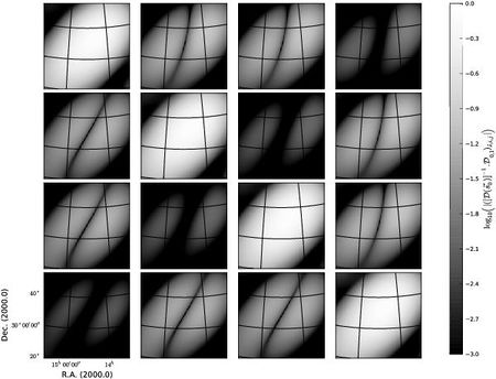
In fig1 normalization is done as, <math>\mathcal{D}_0(\mathbf{s}) = [\mathcal{D}(\mathbf{s}_0)]^{-1} . \mathcal{D}(\mathbf{s})</math>, where <math>\mathbf{s}_0</math> is the phase center.
After normalization, the dipoles projected on the sky are orthogonal at the phase center (off-diagonal terms of the Mueller matrix is zero there). As we go further away from the center, the off-diagonal terms become more and more significant. At a few degrees from the phase center, off-diagonal terms can be as high as 10%.
For the total set of visibilities over all baselines, times and frequencies,
- <math>\mathbf{V} = \mathcal{A}.\mathbf{I} + \epsilon</math>
- <math>\epsilon</math> is the thermal noise.
- <math>\mathcal{A} = \mathcal{W} \mathcal{S} \mathcal{F} \mathcal{D}</math>
To estimate follow the sky least square solution:
- <math>\hat{\mathbf{I}} = (\mathcal{A}^H . \mathcal{A})^{-1} . \mathcal{A}^H . \mathbf{V}</math>
- <math>\mathcal{A}^H . \mathbf{V}</math> is the <math>4N_{pix}</math> dirty image.
- <math>(\mathcal{A}^H . \mathcal{A})^{-1}</math> is the image plane deconvolution matrix, affected by DDEs.
- <math>\mathcal{A}^H . \mathcal{A}</math> is the instrumental response to a source centered on the location of the xth pixel, evaluated at the yth pixel.
But the DDEs can be separated from the rest of the terms as, <math>\mathcal{A}^H . \mathcal{A} = \mathcal{D}^H \mathcal{P} \mathcal{D}</math> where <math>\mathcal{P} = \mathcal{W}^H \mathcal{S}^H \mathcal{F}^H \mathcal{W} \mathcal{S} \mathcal{F}</math>. Thus for a given baseline-frequency block:
- <math>[\mathcal{A}^H . \mathcal{A}](x,y) = \sum\limits_{t,\nu,pq} p_{t,\nu,pq}(x,y) \mathcal{D}_{t,\nu,pq}^H(y) \mathcal{D}_{t,\nu,pq}(x)</math>
Assuming DDEs are constant enough in a given time, frequency, and baseline block:
- <math>[\mathcal{A}^H . \mathcal{A}](x,y) \sim N_{t,\nu,pq} p(x,y) \bar{\mathcal{D}^H \mathcal{D}}(x,y) </math>
[The major cycle computes model and residual visibilities, grids them via convolutional resampling, and Fourier transforms the result to form a residual (or dirty) image. This image is interpreted as the convolution of the sky brightness distribution with the PSF of the instrument, and the minor cycle deconvolves the PSF from the current residual image to create a model image.]
Implementation of A-projection for LOFAR
Tasse+ implemented the Bhatnagar A-projection algorithm on top of the traditional Cotton-Schwab CLEAN algorithm as,
- <math>\hat{\mathbf{I}}^{n+1} = \hat{\mathbf{I}}^{n} + \Phi . \mathcal{A}^H (V - \mathcal{A}\hat{\mathbf{I}}^{n})</math>
- <math>\mathcal{A}^H (V - \mathcal{A}\hat{\mathbf{I}}^{n})</math> is the residual dirty image, computed via the major cycle of CLEAN+A-projection.
- <math>\Phi</math> is a non-linear operator that estimates the deconvolved sky from the residual dirty image.
To compute this residual dirty image, first predict (degridding step), then subtract predicted visibilities from the observed ones. A-projection does this by applying <math>\mathcal{A}</math> on the model sky by seperating the phase terms as,
- <math>V_{pq}^{t,\nu} = \sum\limits_{j=1}^4 \left[ \mathcal{F} (\mathcal{D}_{pq}^{t,\nu}(i,j,\mathbf{s}) W(w,\mathbf{s})) \ast \mathcal{F} (\mathbf{I}_j(l,m)) \right]</math>
- <math>V_{residual} = \mathbf{V} - \mathcal{A}\hat{\mathbf{I}}^N</math>
Applying <math>\mathcal{A}</math> on this residual and gridding them back gives the residual dirty image that is used in the iteration of the first equation of this part.
Further reading
- Bhatnagar et al. (2008): A-projection allows imaging taking all DDEs into account.
- Heald et al. (2010): LOFAR observing process and the pipeline architecture.

